RSS

Author Archives: visualign

Unknown's avatar

About visualign

Visualize Data. Improve Performance.

Self-publishing to Apple bookstore

Self-publishing to Apple bookstore

Over the last couple of weeks I finished writing the book about my adventure of a lifetime: Panamerican Peaks, cycling from Alaska to Patagonia and climbing the highest mountain of every country along the way. By now I have successfully self-published the book to the Apple bookstore. This post gives a recap of the steps involved in that process, with a focus on the tools, logistics and finally some numbers and sales stats.

Disclaimer: In my personal life I am an avid Apple fan, and this post is heavily biased towards Apple products. In particular, the eBook is only available for the iPad. So the tools and publishing route described below may not be for everybody, but the process and lessons learnt may still be of interest.

Path to self-publishing on Apple bookstore

Creating Content

The first step is obviously to create, select and edit the content of the book. During the actual trip I tried documenting my experiences via the following:

  • Taking about 10,000 photos with digital camera (Olympus and Panasonic)
  • Taking daily notes with riding or climbing stats (on iPhone or NetBook)
  • Shooting about 200 video clips (Flip Mino)
  • Uploading photos (to Picasa) and videos (to YouTube)
  • Writing posts on my personal Blog

In the months after coming home I refined some of the above material. Using iMovie I created ~ 5 min long movies based on video clips, photos and map animations, typically with some iTunes song in the background and a bit of explanatory text or commentary. I shared those videos on my personal Blog and on my Panamerican Peaks YouTube channel.

I loaded all photos into Aperture on our iMac and tagged and rated them. That allowed me to organize them by topic or as required. The ‘Smart Folders’ feature of Aperture comes in handy here, as it allows to set up filters and select a subset of photos without having to copy them. For example, if I wanted photos rated 4 stars or higher related to camping, or photos of mountains in Central America, I just needed to create another Smart Folder. This was very useful for example for the Panamerican Peaks Synopsis video which features quick photo sets by topics (cycling, climbing, camping, etc.).

Google Earth proved to be a very useful tool as I could easily create maps of the trip based on the recorded GPS coordinates from my SPOT tracker. One can even retrace the trip in often astonishing detail thanks to Google Street View. For example, in many places along the Pacific Coast I can look at campgrounds or road-side restaurants where I stopped during my journey. I even created a video illustrating the climbing route on Mount Logan from within Google Earth.

The heart and soul of any book is of course the story and the text used to tell it. I created multiple chapters using MS Word because I am so used to it, but one can of course use any modern text writing tool. In addition, I created some slides for presentations I gave last summer using Keynote.

Book Layout

Once all the ingredients were available, it was time to compose the actual book. As I had decided to build an eBook for the iPad I used Apple’s new iBooks Author tool on my MacBook Pro. This meant choosing the layout and including the text and media. iBooks provides a few interactive widgets and accepts all widgets that can be installed into the OS X dashboard. This in particular allowed me to link to the various YouTube videos. I could always get a preview of the book copied out to my attached iPad 2.

After many weeks of busy work putting the finishing touches on the book and adding various edits from a few trusted friends I got to the point where I needed to figure out how to get the book published in Apple’s bookstore. There are two steps required here:

  1. Creating a developer account with Apple via iTunes Connect
  2. Managing one’s content via iTunes Producer

The creation of the account is fairly straightforward through the web browser. To get started, I visited Apple’s Content Provider FAQ page and filled out an application. One submits basic information such as name, address, tax ID, credit card information, and ties it all to an existing Apple account. It can take a while. I never received the account validation email I was promised. So after a few days I started inquiring in Apple’s support forum. This had happened to others. Finally I just tried connecting via web browser to itunesconnect.apple.com and it worked – I had an account to publish from.

The packaging of all material and uploading is done via the free iTunes Producer app on the Mac. iBooks Author exports the book in .ibooks format, which becomes part of the iTunes Producer package. One can also provide a free sample for the book. This can be any subset or variation of the full book, unlike with Amazon’s bookstore, where the free sample is always the first N pages.

Next, one needs to provide additional metadata such as book category, description, author name, optional sample screen shots etc. One also has to provide an ISBN (International Standard Book Number) for the book. These can be obtained from publishers or directly purchased from Bowker. This stems from the need to catalogue and identify physical books in inventory or libraries, but seems a bit anachronistic for electronic books. The prices for ISBNs are very high, especially for small volumes (1 for $125, 10 for $250, 100 for $500, 1000 for $1000). But since Bowker has a monopoly in the US you don’t have a choice in that matter. This expense seemed to be the only marginal upfront cost to publishing the book (aside from the tools to create the content).

Finally one can determine the pricing and the markets where the content is to be sold. Apple follows the agency model of book publishing: As author you get to set the price. As distributors they take a share of your proceeds, here 30%. (By contrast, in the wholesale model you sell to the distributor at a discount, say 50% of the suggested retail price; the seller has sole discretion to set the price.)

Book Review

Much has been written about the very restrictive terms and conditions Apple puts on authors using their iBooks Author tool. Essentially it locks you in as an author to sell only through Apple. For many authors that is not a viable option. It also allows Apple to reject your work at their sole discretion. So as an author you are completely at the mercy of Apple’s review process.

Apple is also strict with enforcing certain rules regarding the content it allows you to sell. For example, your book cannot contain any links to YouTube videos or Amazon books. They rejected my first revision with YouTube links and suggested to embed all videos. This would have bloated the download size of the book by more than 1 GB. As a compromise, I created short 1 min teaser versions of all videos and included those. At the end they display a screen to go to the companion website (my personal Blog) for the full versions.

After 3 revision cycles and about a week later I finally had my book on sale in 24 countries around the world, for $9.99 or the equivalent in Euro or other countries’ currencies.

Book Marketing

Publishing is not selling. Here are some of the things I did to promote my own book:

  • Email – Customized note to Hotmail contacts (~ 300 contacts)
  • Twitter – Tweets and direct messages to influencers for retweets (~ 2000 followers)
  • FaceBook – My daughter posted on her wall (~ 1000+ friends)

Sending the emails was not without hiccups. I used MS Word and Outlook to do a mail merge with text blocks and individual text from an Excel spreadsheet. First, the Mail Merge Filter condition dialog has a bug which replicates the last AND condition and adds it as an OR condition. This screws up your filter and ends up selecting lots of folks you didn’t mean to. I found this bug during a test with the first 5 addresses. (I sent them each an apologetic email explaining this.) Then after I did the filtering all in the spreadsheet it worked and Outlook cranked out the emails. After a short while, Hotmail decided that my account had apparently been hacked and used for spam, so they locked my account down! In a way this is good, but I didn’t consider my carefully crafted and personalized emails spam. So I had to change my password and unlock my account again.
The email was very effective. I got lots of positive responses and a few folks decided to buy right away. I had sold my first copy. Every journey of 1000 miles starts with a single step.

As a result of my daughter posting the news on Facebook I noticed a spike (4x average) in the views of my Blog and Book page. I also offered promo codes for free book download to influential twitter users if they would retweet the book announcement to their followers. Within a couple of days a handful of them accepted the offer and retweeted, which exposed the tweet to a total of 2,000+ followers.

I had emailed the Apple bookstore, and to my delight they actually featured my book in their Travel & Adventure category.

My book featured in Apple’s bookstore, Travel & Adventure section

Book Sales

With all these promotion efforts I couldn’t wait until the next morning to see the sales numbers. (iTunes Connect updates their sales numbers only once a day.) I had the first ratings and reviews come in, all at 5-stars. Naturally, I hoped to see the sales numbers go up. After all, I had reached hundreds, if not thousands of people, most of which either know me or are somewhat interested in adventure. The result? Tiny sales numbers. To date after one week I have sold 14 copies, with a maximum of four (4) copies per day. At my $10 price and 70% share this amounts to just under $100 for the first week. Not exactly enough to retire on.

I’ll revisit this topic at some point in the future when I have more data. Obviously, the iPad is just a fraction of the entire book market with Kindle, Nook and other devices. (Although, the iBook looks much better on the iPad than on many other readers, in particular the smaller black & white e-Ink display Kindle readers.) While the selection of titles seems comparable on Apple’s and Amazon’s bookstores, about 1.35 million each (see a spreadsheet of my recent sample here), there don’t appear to be many shoppers in Apple’s bookstore. Of course, Travel & Adventure is only a small fraction of the book market. But even there, on a day where I sold two copies my book briefly ranked 30.th in the Top Charts. 30.th out of 11,800 titles (in Travel & Adventure)! That means the other 11,770 titles sold even less than mine (i.e. one or none) during the sampling time interval. Book sales appear very unevenly distributed, another case of huge online inequality.

But more importantly, most of the people reached by my promotional efforts don’t engage to the level of actually following the links, downloading the sample and finally buying the book. From my experience, one needs to reach more than 100 people for every one book sold. Fellow adventure traveller and author Andrew Hyde – whose book coincidentally is featured just above mine in the screen-shot above – has recently written about his book sales here. His stats show a similar small fraction of sales to views. I just don’t have the millions of Twitter followers to generate meaningful sales this way!

 
1 Comment

Posted by on June 21, 2012 in Recreational


Tags:

Visualign Blog – View Stats for first year and a half

Visualign Blog – View Stats for first year and a half

I started this Data Visualization Blog back at the end of May 2011. WordPress provides decent analytics to measure things like views, referrer, clicks, etc. The built-in stats show bar charts by day/week/month, views by country, top posts and pages, search engine terms, comments, followers, tags and so on. I have accumulated the view data and wanted to share some analysis thereof.

At this point there are 17,000 views and 56 posts (about 1 post per week). The weekly views have grown as follows:

Weekly Views of Visualign Blog

The WordPress dashboard for monthly views looks like this:

Assuming an exponential growth process this amounts to a doubling roughly every 3 months. This may not sound like much, but if it were to continue, it would lead to a 16x increase per year or a 4096x increase in 3 years. Throughout the first year this model has been fairly accurate and allowed to predict when certain milestones would be reached (such as 10k views, reached in Apr-2011 or 100k views, predicted by Jan-2013).

However, the underlying process is not a simple exponential growth process. Instead it is the result of multiple forces, some increasing, some decreasing, such as level of interest of fresh content for target audience, rather short half-life of web content, size of audience, frequency of emails or tweets with links to the content etc. So I expect growth to slow down and consequently the 100k views milestone to be pushed out past Jan-2013.

Views come from some 112 countries, albeit very unevenly distributed.

Views by Country (10244 views since Feb-25, 2012)

The Top 2 countries (United States and United Kingdom) contribute nearly half of the views, the Top 10 (9%) countries nearly 75% of all views. The fairly high Gini index of this distribution (~0.83) indicates strong dependency on just a few countries. The only surprise for me in the Top 10 list was South Korea, ranking fifth and slightly ahead of India. Germany is probably a bit over-represented due to my German business partner (RapidBusinessModeling) and related network.

Views by country with Top 10 list

One interesting analysis comes from looking at the distribution of views over weekdays. Not every weekday is the same. Thursdays are the busiest, Saturday the quietest days. After a little more than one year, averaging over some 56 weeks, the distribution looks like this.

Weekday variation of Blog views averaged over 1st year

Of course, time zone boundaries may cause some distortions here, but it looks like the view activity builds during the week until it hits a peak on Thursday. Then it falls sharply to a low on Saturday, and builds from there again. This fits with intuition: One would expect the weekend days to be low as well as Monday and Friday to be lower than the mid-week days. It’s tempting to correlate that with the amount of work or research getting done by professionals. The underlying assumption is that people discover or revisit my Blog when it fits into their work.

A large fraction (> 65%) of referrals comes from search engines. Within those, it’s mostly Google (>90% summed across many countries) with just a small amount of others like Bing. It’s safe to say that without Google search my Blog would have practically no views. Chances are that your first exposure to this Blog came from a Google search as well. One unexpected insight for me was to see a high ratio of image to text searches, typically 3:1 or 4:1. In some ways it shouldn’t be surprising that a blog on data visualizations gets discovered more often by searching for visual elements than for text. It also jibes with the enormous growth of image related sites such as Instagram or Pinterest. I just would not have expected the ratio to be that high.

The beginning is always slow. But any exponential growth sooner or later leads to rather large numbers. So the real question is how one can keep the exponential growth process going? I’d love to hear your comments. If you want to compare this against your own Blog stats, I have shared the underlying data as a Google doc here. I have no idea how this compares to other blog stats in similar domains. If you know of any other public Blog stats analysis, please comment with a pointer below. Thanks.

Addendum 7/11/2012: Today my Blog reached 20,000 views. I noticed over the last few weeks that the deviation from an exponential growth model was getting quite large. For an exponential trend line R² = 0.9886.

Daily views with 20,000 total view milestone

When instead modeling the weekly views on a linear growth rate, this gives the total views a quadratic growth. Curve fitting the total views with a 2nd order polynomial yields a very good fit (R² = 0.9977).

Total views growth curve with quadratic curve fit

Linear growth of weekly views is compatible with approximately linear increase in content (steady frequency of about 1 post / week) and thus increased chance of Google search indexing new content (with Google search the main source of view traffic). Quadratic growth of total views is also nonlinear, but far slower than exponential growth. For example, the 100,000 view milestone is now projected to be reached in 08/2013 instead of in 01/2013, i.e. in 13 months as compared to 7 months.

Addendum 11/1/2012: The Blog reached 30000 views on Oct-19 and here is a chart of the monthly views through Oct-2012:

Monthly Blog views through Oct-2012

August and September have been slow, presumably seasonal variation. I also didn’t post between late August and mid October. The view data of the last couple of months no longer support the theory of significant growth in view frequency. Instead, multiple dynamic factors come into play. At times views spike due to a mention or a post of temporary interest – such as the recent post on visualizing superstorm Sandy. But such spikes quickly fade away according to the very limited half-life of web information these days. The undulating 4 week trailing average in weekly views below visualizes this clearly. The net effect has been a plateau in view frequency around 3000 per month.

Weekly Views with average Nov 2012

I continue to see most of the referrals coming from Google searches, still with a majority of those being image searches. Engagement growth has been anemic, with relatively few comments, back links or other forms of engagement. It seems to me that growth proceeds in phases, with growth spurts interspersed by plateaus of varying length. One such growth spurt has been reported by Andrei Pandre on his Data Visualization Blog through the use of Google+. Perhaps it’s time to extend this Blog to Google+ as well.

Variation of views by weekday

With regard to variation of views by weekday, the qualitative pattern remains. Tuesday is now emerging as the day with the most views, with Monday, Wednesday, and Thursday slightly behind, but still above average. Friday is slightly below average, Saturday is the lowest day with only half the views and Sunday in between.

I’m not sure whether to conclude from that that important posts should be published on a particular weekday. Again, most views come from Google searches and are accumulated over time, so perhaps only the height of the initial spike will vary somewhat based on the publishing weekday.

 
Leave a comment

Posted by on June 12, 2012 in Scientific


Venn Diagrams

Venn Diagrams

The private library Blog had a post with some word play relating to sound, spelling and meaning of words in the English language. From their post on Homographic Homophones:

English is one of the most difficult languages in the world for a non-native speaker to learn.  One of the reasons why this is so is that English has a large number of words that are pronounced the same as other words (i.e., they are homophones) even though they have quite different meanings.  Homophones such as parepair and pear, for example, have the same pronunciation but are spelled differently and have different meanings (heterographic homophones).  Other homophones — tender (locomotive),tender (feeling) and tender (resignation), for instance — are spelled the same and pronounced the same (homographic homophones) but have different meanings (i.e., they are homonyms).

Got all that?  Wikipedia has a nice Venn diagram that may help you sort it out:

Venn Diagram displaying meaning, spelling, and pronunciation of words (Source: Wikipedia)

Of course, you could also list the above combinations in a table. If you’re interested, Carol Moore has done just that on her Buzzy Bee riddle page.

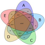
A beautifully symmetric 5 set Venn diagram drawn from ellipses has been proposed by Branko Grünbaum and drawn by Wikipedia contributor Cmglee:

Symmetrical_5-set_Venn_diagram (Source: Wikipedia)

Such set-based diagrams invite a more mathematical notation. Cmglee annotates his image with this snippet:

Labels have been simplified for greater readability; for example, A denotes A ∩ Bc ∩ Cc ∩ Dc ∩ Ec (or A ∩ ~B ∩ ~C ∩ ~D ∩ ~E), while BCE denotes Ac ∩ B ∩ C ∩ Dc ∩ E (or ~A ∩ B ∩ C ∩ ~D ∩ E).

If you search the Wolfram Demonstration Project for ‘Venn Diagram’, you get several interactive diagrams.

Venn Diagram Demonstration Projects (Source: Wolfram Demonstration Project)

These diagrams are interactive. For example, they allow you to click on any subset and then have that set highlighted and the corresponding mathematical set notation displayed accordingly. Interesting and fun to learn.

Speaking of fun: Venn diagrams are also effectively used in many different areas, two of which I’d like to leave you with here:

Data Science Venn Diagram (Source: drewconway.com)

And last but not least, Stephen Wildish’s Pancake Venn Diagram:

 
Leave a comment

Posted by on June 10, 2012 in Linguistic, Scientific


Tags: , , ,

Graphic comparing highest mountains

Graphic comparing highest mountains

In mountaineering, 8000m peaks are the ultimate test of high-altitude climbing. It so happens that there are 14 Eight-thousanders. In 1986 Reinhold Messner became the first person to have climbed all 14 8000m peaks. It has become a coveted trophy of mountaineering, with only about 30 people having done so since.

A different, but somewhat related challenge is to climb the highest mountain on every continent, the so-called Seven Summits. This was first completed by Dick Bass in 1985. It has become a more mainstream mountaineering challenge, and about 300 people have repeated that feat. That has also lead to significant and often problematic overcrowding on those seven summits.

Interestingly, it was noted that the second highest mountain on each continent is typically harder to climb than the highest. Hence yet another challenge was born to complete the first ascent of the Seven Second Summits. Hans Kammerlander claims to have done so in 2010 – although some doubts have arisen regarding whether he stood on the right summit on Mount Logan, Canada. Others have suggested combining the Seven Summits and the Seven Second Summits, giving again 14 peaks.

On the Wikipedia page I found an interesting graphic comparing the 14 Eight-thousanders with the Seven + Seven Second Summits. It was created by Cmglee and shared on the Wikipedia page.

Comparison of highest mountains (Source: Wikipedia)

This is an interesting chart, created as .svg file and thus rendering in high definition on large wide-format screens. It is also interesting to follow the revision history on the talk page and the suggestions about coloring and labeling coming from interested readers. In some ways, this shows how published charts can be improved collaboratively. Contributor ‘Cmglee’ has contributed several .svg graphics to Wikipedia as per the User talk page, including a 5-set Venn diagram, life-expectancy bubble charts and Earthquake intensity bubble charts.

I have a personal interest in mountaineering. In 2009-2010 I embarked on my own adventure of a lifetime called the ‘Panamerican Peaks’. Cycling between Alaska and Patagonia (Panamerican Highway) and Climbing the highest mountain of every country along the way. You can find out more about that adventure on my Panamerican Peaks website. Coincidentally, there are a minimum of 14 countries and peaks in that set as well: United States, Canada, Mexico, Guatemala, El Salvador, Honduras, Nicaragua, Costa Rica, Panama, Colombia, Ecuador, Peru, Chile, Argentina.

Position and elevation of 14 Panamerican Peaks

Prior to starting my adventure journey I had mapped out the height of those 14 mountains. Interestingly, except for a few peaks in Central America, the country high-points get higher the further North or South they are located.

Heights of 14 Panamerican Peaks

Four of those peaks are included in the Seven (Second) Summit lists above: Denali, Logan (North America) and Aconcagua, Ojos (South America). It would be great to include the other 10 Panamerican Peaks in a similar graphic. About time for me to look into generating .svg graphics…

And sure enough, Wikipedia contributor Cmglee provided me with a version of the above .svg chart comparing the 14 Panamerican Peaks with the 14 Seven (Second) Summits as follows:

Comparison of 14 Panamerican Peaks with Seven (Second) Summits

Thanks to Cmglee for the quick turn-around.

 
1 Comment

Posted by on June 4, 2012 in Recreational


Connectograms and Circos Visualization Tool

Connectograms and Circos Visualization Tool

Yesterday (May 16) the Public Library of Science (PLoS) published a fascinating article titled “Mapping Connectivity Damage in the Case of Phineas Gage“. It analyzes the brain damage which the famous trauma victim sustained after an accident drove a steel rod through his skull. Railroad worker Phineas Gage survived the accident and continued to live for another 12 years, albeit with significant behavioral changes and anomalies. Those changes were severe enough for him to have to discontinue his work and also get estranged from his friends who stated he was “no longer Gage”. This has become a much studied case about the impact of brain damage on behavior anomalies. Since the accident happened more than 150 years ago there are no autopsy data or brain scans from Phineas Gage’s brain. So how did the scientists reconstruct the likely damage?

Since a few years there has been interest in the human connectome. Just like the genome is a map of human genes, the connectome is a map of the connectivity in the human brain. The human brain is enormously complex. Most estimates put the number of neurons in the hundreds of billions and the synaptic interconnections in the hundreds of trillions! Using diffusion weighted (DWI) and magnetic resonance imaging (MRI) one can identify detailed neuron connectivity. This is such a challenging endeavor that it drives the development of many new technologies, including the data visualization. The image resolution and post-processing power of modern instruments is now large enough to create detailed connectomes that show major pathways of neuronal fibers within the human brain.

The authors of the Laboratory of Neuro Imaging (LONI) in the Neurology Department at UCLA have studied the connectomes of a population of N=110 healthy young males (similar in age and dexterity to Phineas Gage at the time of his accident). From this they constructed a typical healthy connectome and visualized it as follows:

Circular representation of cortical anatomy of normal males (Source: PLoS ONE)

Details of the graphic are explained in the PLoS article. The outermost ring shows the various brain regions by lobe (fr – frontal, ins – insula etc.). The left (right) half of the connectogram figure represents the left (right) hemisphere of the brain and the brain stem is at the bottom, 6 o’clock position of the graph.

Connectograms are circular representations introduced by LONI researchers in their NeuroImage article “Circular representation of human cortical networks for subject and population-level connectomic visualization“:

This article introduces an innovative framework for the depiction of human connectomics by employing a circular visualization method which is highly suitable to the exploration of central nervous system architecture. This type of representation, which we name a ‘connectogram’, has the capability of classifying neuroconnectivity relationships intuitively and elegantly.

Back to Phineas Gage: His skull has been preserved and is on display at a museum. Through sophisticated spatial and neurobiological reasoning the researchers reconstructed the pathway of the steel rod and thus the damaging effects on white matter structure.

Phineas Gage Skull with reconstructed steel rod pathway and damage (Source: PLoS ONE)

Based upon this geospatial model of the damaged brain overlaid against the typical brain connectogram from the healthy population they created another connectogram indicating the connections between brain regions lost or damaged in the accident.

Mean connectivity affected in Phineas Gage by the accident damage (Source: PLoS ONE)

From the article:

The lines in this connectogram graphic represent the connections between brain regions that were lost or damaged by the passage of the tamping iron. Fiber pathway damage extended beyond the left frontal cortex to regions of the left temporal, partial, and occipital cortices as well as to basal ganglia, brain stem, and cerebellum. Inter-hemispheric connections of the frontal and limbic lobes as well as basal ganglia were also affected. Connections in grayscale indicate those pathways that were completely lost in the presence of the tamping iron, while those in shades of tan indicate those partially severed. Pathway transparency indicates the relative density of the affected pathway. In contrast to the morphometric measurements depicted in Fig. 2, the inner four rings of the connectogram here indicate (from the outside inward) the regional network metrics of betweenness centrality, regional eccentricity, local efficiency, clustering coefficient, and the percent of GM loss, respectively, in the presence of the tamping iron, in each instance averaged over the N = 110 subjects.

The point of the above quote is not to be precise in terms of neuroscience. Experts can interpret these images and advance our understanding of how the brain works – I’m certainly not an expert in this field, not even close. The point is to show how advances in imaging and data visualization technologies enable inter-disciplinary research which just a decade ago would have been impossible to conduct. There is also a somewhat artistic quality to these images, which reinforces the notion of data visualization being both art and science.

The tool used for these visualizations is called Circos. It was originally developed for genome and cancer research by Martin Krzywinski at the Genome Sciences Center in Vancouver, CA. Circos can be used for circular visualizations of any tabular data, and the above connectome visualization is a great application. Martin’s website is very interesting in terms of both visualization tools as well as projects. I have already started using Circos – which is available both for download and in an online tableviewer version – for some visualization experiments which I may blog about in the future.

 
7 Comments

Posted by on May 17, 2012 in Scientific


Tags: , , , ,

Faceplant with Facebook?

With the Facebook IPO coming up this Friday there is a lot of attention around its business model and financials. I’m not an expert in this area, but my hunch is that a lot of people will lose a lot of money by chasing after Facebook shares. Why?

I think there are two types of answers. One from reasoning and one from intuition.

For reasoning one needs to look at a more technical assessment of the business model and financials. Some have written extensively about the comparative lack of innovation in Facebook’s business model and core product. Some have compared Facebook’s performance in advertising to Google – the estimates are that Google’s ad performance is 100x better than that of Facebook. Some have pointed out that many of Facebook’s core metrics such as visits/person, pages/visit or Click-Through-Rates have been declining for two years and go as far as calling this the Facebook ad scam. One can question the wisdom of the Instagram acquisition, buying a company with 12 employees and zero revenues for $1B. One can question the notion that the 28 year old founder will have 57% of the voting rights of the public company. One could look at stories about companies discontinuing their ad Facebook efforts such as the Forbes article about GM pulling a $10m account because they found it ineffective. The list goes on.

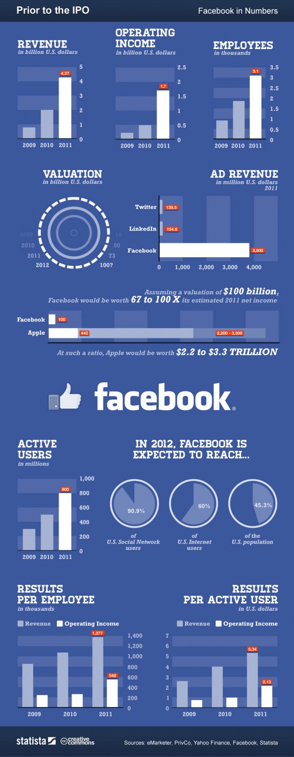
Here is a more positive leaning infographic from an article looking at “Facebook: Business Model, Hardware Patents and IPO“:

Analysis Infographic of pre-IPO Facebook (source: Gina Smith, anewdomain.net)

To value a startup at 100x last year’s income seems just extremely high – but then Amazon’s valuation is in similarly lofty territory. As for reasoning and predicting the financial success of Facebook’s IPO, people can cite numbers to justify their beliefs both ways. At the end of the day, it’s unpredictable and nobody can know for sure.

The other answer to why I am not buying into the hype is more intuitive and comes from my personal experience. Here is a little thought experiment as to how valuable a company is for your personal life: Imagine for a moment if the company with all its products and services would disappear overnight. How much of an impact would it have for you as an individual? If I think about companies like Apple, Google, Microsoft, or Amazon the impact for me would be huge. I use their products and services every day. Think about it:

No Apple = no iPhone, no iPad, no iTunes music on the iPod or via AppleTV on our home stereo. That would be a dramatic setback.

No Google = no Google search, no GMail, no YouTube, no Google maps, no Google Earth. Again, very significant impact for me personally. Not to mention the exciting research at Google in very different areas such as self-driving vehicles.

No Facebook = no problem (at least for me). I deactivated my own Facebook account months ago simply because it cost me a lot of time and I got very little value out of it. In fact, I got annoyed with compulsively looking at updates from mere acquaintances about mundane details of their lives. Why would I care? I finally got around to actually deleting my account, although Facebook makes that somewhat cumbersome (which probably inflates the account numbers somewhat).

I’m not saying Facebook isn’t valuable to some people. Having nearly 1B user accounts is very impressive. Hosting by far the largest photo collection on the planet is extraordinary. Facebook exploded because it satisfied our basic need of sharing, just like Google did with search, Amazon did with shopping or eBay did with selling. But the entry barrier to sharing is small (see LinkedIn, Twitter or Pinterest) and Facebook doesn’t seem to be particularly well positioned for mobile.

I strongly suspect that Facebook’s valuation is both initially inflated – the $50 per account estimate of early social networks doesn’t scale up with the demographics of the massive user base – as well as lately hyped up by greedy investors who sense an opportunity to make a quick buck. My hunch is that FB will trade below its IPO price within the first year, possibly well below. But then again, I have been surprised before…

I’m not buying the hype. What am I missing? Let me know what you think!

UPDATE 8/16/2012: Well, here we are after one quarter, and Facebook’s stock valuation hasn’t done so well. Look at the first 3 month chart of FB:

First 3 month of Facebook stock price (Screenshot of StockTouch on iPad)

What started as a $100b market valuation is now at $43b. One has to hand it to Mark Zuckerberg, he really extracted maximum value out of those shares. It turns out sitting on the sidelines was the right move for investors in this case.

 
2 Comments

Posted by on May 16, 2012 in Financial, Socioeconomic


Tags: , , , , , , ,

Sankey Diagrams

Sankey Diagrams

Whenever you want to show the flow of a quantity (such as energy or money) through a network of nodes you can use Sankey diagrams:

“A Sankey diagram is a directional flow chart where the width of the streams is proportional to the quantity of flow, and where the flows can be combined, split and traced through a series of events or stages.”
(source: CHEMICAL ENGINEERING Blog)

One area where this can be applied very well is that of costing. By modeling the flow of cost through a company one can analyze the aggregated cost and thus determine the profitability of individual products, customers or channels. Using the principles of activity-based costing one can create a cost-assignment network linking cost pools or accounts (as tracked in the General Ledger) via the employees and their activities to the products and customers. Such a Cost Flow can then be visualized using a Sankey diagram:

Cost Flow from Accounts via Expenses and Activities to Products

The direction of flow (here from left to right) is indicated by the color assignment from nodes to its outflowing streams. Note also the intuitive notion of zero-loss assignment: For each node the sum of the in- and outflowing streams (= height of that node) remains the same. Hence all the cost is accounted for, nothing is lost. If you stacked all nodes on top of one another they would rise to the same height. (Random data for illustration purposes only.)

The above diagram was created in Mathematica using modified source code originally from Sam Calisch who had posted it in 2011 here. Sam also included a “SankeyNotes.pdf” document explaining the details of the algorithms encoded in the source, such as how to arrange the node lists and how to draw the streams.

I find these a perfect example of how a manual drawing can go a long ways to illustrate the ideas behind an algorithm, which makes it a lot easier to understand and reuse the source code. Thanks to Sam for this code and documentation. Sam by the way used the code to illustrate the efficiency of energy use (vs. waste) in Australia:

Energy Flow comparison between New South Wales and Australia (Sam Calisch)

Note the sub-flows within each stream to compare a part (New South Wales) against the whole (Australia).

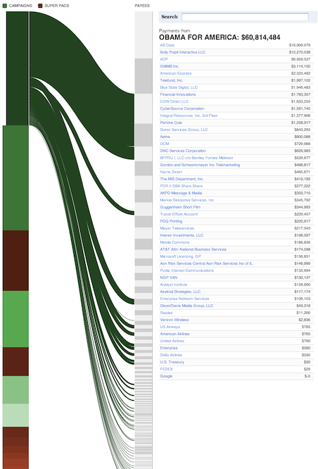
Another interesting use of Sankey Diagrams has been published a few weeks ago on ProPublica about campaign finance flow. This is particularly useful as it is interactive (click on image to get to interactive version).

Tangled Web of Campaign Finance Flow

Note the campaigns in green and the Super-PACs in brown color. The data is sourced from FEC and the New York Times Campaign Finance API. Note that in the interactive version you can click on any source on the left or any destination on the right to see the outgoing and incoming streams.

Finance Flow From Obama-For-America

Finance Flow to American Express

Here are some more examples. Sankey diagrams are also used in Google Flow Analytics (called Event Flow, Goal Flow, Visitor Flow). I wouldn’t be surprised to see Sankey Diagrams make their way into modern data visualization tools such as Tableau or QlikView, perhaps even into Excel some day… Here are some Visio shapes and links to other resources.

 
4 Comments

Posted by on May 14, 2012 in Financial, Industrial


Tags: , , ,

Quarterly Comparison: Apple, Microsoft, Google, Amazon

Quarterly Comparison: Apple, Microsoft, Google, Amazon

Last quarter we looked at the financials and underlying product & service portfolios of four of the biggest technology companies in the post “Side by Side: Apple, Microsoft, Google, Amazon“. With the recent reporting of results for Q1 2012 it is a good time to revisit this subject.

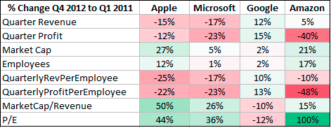
Comparison of Financials Q4 2011 and Q1 2012 for Apple, Microsoft, Google, and Amazon.

Market cap has grown roughly by 25% for both Apple and Amazon, whereas Microsoft and Google only added 5% or less. A sequential quarter comparison can be misleading due to seasonal changes, which impact different industries and business models in a different way. For example, Google’s ad revenue is somewhat less impacted by seasonal shopping than the other companies.

Sequential quarter comparison of financials

Apple and Microsoft seem to be impacted in a similar way by seasonal changes. For Amazon, which already has by far the lowest margin of all four companies, operating income decreased by 40% while it increased its headcount by 17%. This leads to much lower income per employee and with increased stock price to a doubling of its already very high P/E ratio. I’m not a stock market analyst, but Amazon’s P/E ratio of now near 200 seems extraordinarily high. By comparison, the other companies look downright cheap: Apple 8.8, Microsoft 10.5, Google 14.5

Horace Dediu from asymco.com has also revisited this topic in his post “Which is best: hardware, software, or services?“. What’s striking is that all three companies (except Amazon) now have operating margins between 30-40% – very high for such large businesses – with Apple taking the top near 40%. Over the last 5 years, Apple has doubled it’s margin (20% to 40%), whereas Microsoft (35-40%) and Google (30-35%) remained near their levels.

(Source: Asymco.com)

Long term the most important aspect of a business is not how big it has become, but how profitable it is. In that regard Amazon is the odd one out. Their operating income last quarter was about 1% of revenue. Amazon needs to move $100 worth of goods to earn $1. They employ 65,000 people and had revenue of $13.2b last quarter, yet only earned $130m during that time! Apple earns more money just with their iPad covers! Amazon’s strategy is to subsidize the initial Kindle Fire sale and hoping to make money on the additional purchases over the lifetime of the product. In light of these numbers, do you think Amazon has a future with it’s Kindle Fire tablet against the iPad?

But what really struck me about the extreme differences in profitability is this comparison of Apple and Microsoft product lines (source: @asymco twitter):

(source: @asymco twitter)

This shows what an impressive and sustained success the iPhone has been. And the iPad is on track to grow even faster. Horace Dediu guesses that Apple’s iPad will be a bigger profit generator than Windows in one quarter, and a bigger profit generator than Google (yes, all of Google) in three quarters. We will check on those predictions when the time comes…

 
3 Comments

Posted by on May 2, 2012 in Financial, Industrial


Tags: , , , , , ,

Tube Maps

Tube Maps

I just got back from a combined business and vacation trip around Easter to Germany and Austria. In Europe, public transportation is an important part of the infrastructure. Especially in the big cities many people commute daily by train or subway, some even live without a car.

One of the most important pieces of information for train and subway systems is the tube map. It is a schematic transit map showing the lines, stations and connections of the train or subway system. It’s main element is that it abstracts away geographical detail (where is what) and focuses on topological aspects: How do I need to transit to which other line to get to a particular station?

London Tube Map (Source: Wikipedia)

The Wikipedia tube map article details the origins around the London subway system which was called the tube (hence the name for this type of map) dating back to first schematic maps in 1931 by Harry Beck:

“Beck was a London Underground employee who realised that because the railway ran mostly underground, the physical locations of the stations were irrelevant to the traveller wanting to know how to get to one station from another — only the topology of the railway mattered.”

This style of map has been widely adopted and successively refined. Having grown up in Munich and having used its train (S-Bahn) and subway (U-Bahn) system for some 25 years, I came to realize that it is not only a convenient tool for the traveller. It can form the basis of mental models of the topology of a city. The first lines of the Munich S- and U-Bahn system were built for the Olympic Games in 1972. The history and evolution of the train and subway system over the 40 years since has been documented on this website. Let’s look at the tube maps and their evolution in roughly 10 year time intervals.

Munich Tube Map 1971

1971: Note the basic shape of a central track West-East shared by all S-Bahn lines which then fan out radially to the suburbs. The 45° angles help with the text labels and add simplicity to the layout. This simplicity is one key element for such tube maps to become a mental model of the city topology, i.e. of knowing what is where and how to get to it. Note that initially there are only two U-Bahn lines sharing most of their underground tracks.

Munich tube map 1980

1980: The design of the map evolves to “stretch” out the line-graph to both fill out the entire available rectangular space and to free up some more space in the center; here two additional U-Bahn lines require more space, also due to the fact that U-Bahn stations are closer together than S-Bahn stations in the periphery. The Text label “P+R” is introduced to designate Park & Ride facilities at the stations for commuters.

Munich tube map 1992

1992: Some additional U-Bahn lines and stations fill in the center. One of the S-Bahn lines is renamed (S3 -> S8) and extended to the North to connect to the new Munich airport (Erding). Also a few minor map changes (new color scheme, font and legend).

Munich tube map 2001

2001: S1 now also reaches the new airport, which simplifies travel from the Western part of the city and effectively creates a Northern loop. The map changes in the top section to reflect this new topology; this graphically compresses the U-Bahn system in the upper half. A new color (blue) for the stations represents he inner zone. This together with the new text label “XXL” represents tariff boundaries. (A similar approach with blue font color for inner zone station names was dropped after a brief version in 1997; it looked confusing.)

Munich tube map 2012

2012: The current map adds several graphical aspects such as the concentric rings of background color for tariff boundaries, a new font for cleaner look and less line breaks as well as icons for long distance train connections. It also shows some geographic features such as the Isar river and the two lakes in the South-West as well as icons for tourist attractions or land-marks such as the new soccer stadium, the ‘Deutsches Museum’ or the Zoo. For a hi-res map see this pdf file.

Such a sequence shows the evolution of schematic concepts and visual representations over the decades. When you take away some of the simplifying tube map abstractions such as the 45° angle, you get topographical maps like this:

Topographical map of Munich U-Bahn 2010

While such a map gives you a more precise idea of where you are at any given station in the city, it is much harder to remember and to reconstruct in your head. I believe that this simplicity-by-design of modern tube maps makes it such a strong candidate for forming the basis of mental models of city topology.

Here is an interesting variation of the Munich transit system in a so called isochrone map using colors to display transit times say from the center to other city destinations. Robin Clarke created the following map and describes in this post how he did it.

Munich transit system Isochrone Map (Source: Robin Clarke)

A final example of using tube maps in an interactive graphic comes from Tom Carden. He created an applet that lets you click on any of the 200 London subway stations and get a isochronic map showing transit times from that origin to any other station. While not laid out as clean as the Beck-style tube maps, this interactive graphic represents 200 different maps all in one! (Click on the image to get to the interactive version.)

Interactive London Tube Map (Source: Tom Carden)

See also the more recent Blog post London Tube Map for additional examples of graph visualizations using the London underground as illustration object.

As a traveller arriving in an unknown city we often tend to take such subway infrastructure and its documentation for granted. What amazes me is to think about the amount of cumulative work – plan, design, construction, logistics, etc. – that has gone into building such an infrastructure. A few interesting facts about the Munich U-Bahn (subway) system: 6 lines, 100 stations, 103 km, ~ 1 million passengers /day. (Source: Wikipedia). Building a subway costs in the order of $100 million/km, so this represents an investment of about $10 billion! Think about that the next time you try to find your way through a new city…

 
2 Comments

Posted by on April 20, 2012 in Industrial, Recreational


Tags: ,

Khan Academy and Interactive Content in Digital Education

Khan Academy and Interactive Content in Digital Education

Online education has received a lot of attention lately. Many factors have contributed to the rise in online educational content, including higher bandwidth, free video hosting (YouTube), mobile devices, growing and global audiences, improved customization mechanisms (scoring, similarity recommendations), gamification (earning badges, friendly competitions, etc.) and others. Interactivity is an important ingredient for any form of learning.

“I tell you and you forget. I show you and you remember. I involve you and you understand.” [Confucius, 500 BC]

During learning a student forms a mental model of the concepts. Understanding a concept means to have a model detailed enough to be able to answer questions, solve problems, predict a system’s behavior. The power of interactive graphics and models comes from the ability of the student to “ask questions” by modifying parameters and receive specific answers to help refine or correct the evolving mental model.

Digital solutions are bringing innovations to many of these areas. One of the most innovative approaches is the Khan Academy. What started as an experiment just a few years ago by way of recording short, narrated video lessons and sharing them via YouTube with family and friends has grown into a broad-based approach to revolutionize learning. Over the years, founder Sal Khan has developed a large collection of more than 3000 such videos. Backed by prominent endorsers such as Bill Gates the not-for-profit Khan Academy has developed a web-based infrastructure which can handle a large number of users and collect and display valuable statistics for students and teachers. The Khan Academy has received lots of media attention as well, with coverage on CBS 60 minutes, a TED talk and more. The videos have by now been seen more than 130 million times!

Another high profile experiment has been launched in the fall of 2011 at Stanford University, where three Computer Science courses have been made available online for free, including the Introductory Course to Artificial Intelligence by Sebastian Thrun and Peter Norvig. In a physical classroom a professor can teach several dozens to a few hundred students at most. In a virtual classroom these limits are obviously far higher. Exceeding all expectations, some 160.000 students in 190 countries had signed up for this first course!

The basic pillar of online learning continues to be the recorded video of a course unit. The student can watch the video whenever, wherever to learn at his own pace and schedule. One can pause, rewind, replay however often as needed to better understand the content. Of course, if that was the only way to interact, it would be fairly rudimentary. Unlike in a real classroom or with a personal tutor, one can’t ask the teacher in the video a question and receive an answer. One can’t try out variations of a model and see its impact.

Sample Khan Academy Profile Graph

That’s where the tests come in. Testing a concept’s understanding usually involves a series of sample questions or problems which can only be solved repeatedly and reliably with such an understanding. Both Khan Academy and the Stanford AI course have test examples, exams and grading mechanisms to determine whether a student has likely understood a concept. In the Khan Academy, testable concepts revolve around mathematics, where an unlimited number of specific instances can be generated for test purposes. The answers to test questions are recorded and can be plotted.

Khan Academy Knowledge Map of testable concepts

The latter form of interactivity may be among the most useful. The system records how often you take tests, how long it takes you to answer, how often you get the answers right, etc. All this can then be plotted in some sort of dashboard. Both for yourself as individual student, or for an entire class if you are a coach. This shows at a glance where you or your students are struggling and how far along they have progressed.

Concepts are related to one another in a taxonomy so that one gets guidance as to which concepts to master first before building higher level concepts on top of the simpler ones. Statistical models can suggest the most plausible hints of what to try next based on prior observations.

Founder Sal Khan deserves a lot of respect for having almost single-handedly having recorded some 3000+ video lessons and changing the world of online education so much for the better with his not-for-profit organization. From an interactive content perspective, imagine if at the end of some Khan video lessons you could download an underlying model, play with the parameters and maybe even extend the model definition? I know this may not be feasible in all taught domains, but it seems as if there are many areas ripe for such additional interactivity. We’ll look at one in the next post.

 
1 Comment

Posted by on March 26, 2012 in Education


Tags: , , ,