RSS

Tag Archives: Mathematica

Olympic Medal Charts

Olympic Medal Charts

The 2012 London Olympic Games ended this weekend with a colorful closing ceremony. Media coverage was unprecedented, with other forms of competition around who had the most social media presence or which website had the best online coverage of the games.

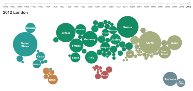
In this post I’m looking at the medal counts over the history of the Olympic Games (summer games only, 27 events over the last 116 years, no games in 1916, 1940, and 1944). Nearly 11.000 athletes from 205 countries competed for more than 900 medals in 302 events. The New York Times has an interactive chart of the medal counts on their London 2012 Results page:

Bubble size represents the number of medals won by the country, bubble position is roughly based on a world map and bubble color indicates the continent. Moving the slider to a different year changes the bubbles, which gives a dynamic grow or shrink effect.

Below this chart is a table listing all gold, silver, bronze winners for each sport in that year, grouped by type of sport such as Gymnastics, Rowing or Swimming. Selecting a bubble will filter this to entries where the respective country won a medal. This shows the domination of some sports by certain countries, such as Diving (8 events, China won 6 gold and 10 total medals) or Cycling – Track (10 events, Great Britain won 7 gold and 9 total medals). In two sports, domination by one country was 100%: Badminton (5 events, China won 5 gold and 8 total medals), Table Tennis (4 events, China won 4 gold and 6 total medals).

There is also a summary table ranking the countries by total medals. For 2012, the United States clearly won that competition, winning more gold medals (46) than all but 3 other countries (China, Russia, Britain) won total medals.

Top 10 countries for medal count in 2012

Of course countries vary greatly by population size. It is remarkable that a relatively small nations such as Jamaica (~2.7 million) won 12 medals (4, 4, 4), while India (~1.25 billion) won only 6 medals (0, 2, 4). In that sense, Jamaica is about 1000x more medal-decorated per population size than India! In another New York Times graphic there is an option to compare medal count adjusted for population size, i.e. with the medal count normalized to a standard population size of say 100 million.

Directed graph comparing medal performance adjusted for country size

Selecting any node in this graph will highlight countries with better, worse or comparable relative medal performance. (There are different ways to rank based on how different medals are weighted.)

The Guardian Data Blog has taken this a step further and written a piece called “alternative medals table“. This post not only discusses multiple factors like population, GDP, or number of athletes and how to deal with them statistically; it also provides all the data and many charts in a Google Docs spreadsheet. One article combines GDP adjustment with cartographical mapping across Europe:

Medals GDP Adjusted and mapped for Europe

If you want to do your own analysis, you can get the data in shared spreadsheets. To do a somewhat more historic analysis, I used a different source, namely Wolfram’s curated data source accessible from within Mathematica. Of course, once you have all that data, you can examine it in many different directions. Did you know that 14853 Olympic medals were awarded so far in 27 summer Olympiads? The average was 550 medals, growing about 29 medals per event with nearly 1000 awarded in 2008 and 2012.

A lot of attention was paid to who would win the most medals in London. China seemed in contention for the top spot, but in the end the United States won the most medals, as it did in the last 5 Olympiads. Only 7 countries won the most medals at any Olympiad. Greece (1896), France (1900), the United Kingdom (1908), Sweden (1912), and Germany (1936) did so just once. The Soviet Union (which no longer exists) did it 8 times. And the United States did it 14 times. China, which is only participating since 1984, has yet to win the most medals of any Olympiad.

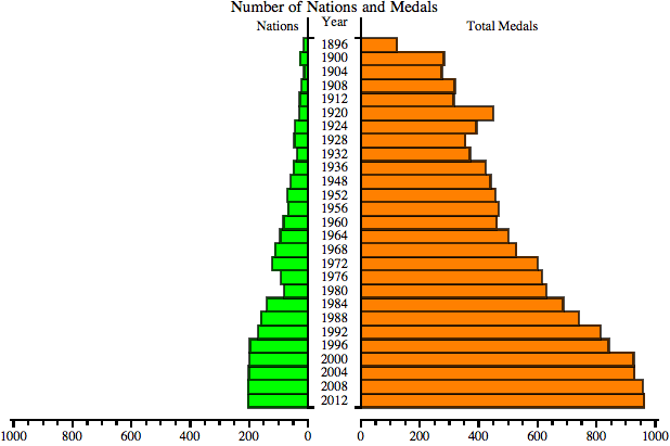
Aside from the top rank, I was curious about the distribution of medals over all countries. Both nations and events have increased, as is shown in the following paired bar chart:

Number of participating nations and total medals per Summer Games

The number of nations grew steadily with only two exceptions during the thirties and the seventies; presumably due to economic hardship many nations didn’t want to afford participation. 1980 also saw the Boycott of the Moscow Games by the United States and several other delegations over geopolitical disagreements. At just over 200 the number of nations seems to have stabilized.

The number of medals depends primarily on the number of events at each Olympiad. This year there were 302 events in 26 types of Sports. Total medal count isn’t necessarily exactly triple that since in some events there could be more than 1 Bronze (such as in Judo, Taekwondo, and Wrestling). Case in point, in 2012 there were 968 medals awarded, 62 more than 3 * 302 events.

What is the distribution of those medals over the participating nations? One measure would be the percentage of nations winning at least some medals. Another measure showing the degree of inequality in a distribution is the Gini index. Here I plotted the percentage of nations medaling and the Gini index of the medal distribution over all participating nations for every Olympiad:

Percentage and Gini-Index of medal distribution by nations

Up until 1932 3 out of 4 nations won at least some medals. Then the percentage dropped down to levels around 40% and lower since the sixties. That means 6 of 10 nations go home without any medals. During the same time period the inequality grew from Gini of about .65 to near .90 One exception were the Third Games in 1904 in St. Louis. With only 13 nations competing the United States dominated so many sports to yield an extreme Gini of .92 All of the last five Games resulted in a Gini of about .86, so this still very large amount of medal winning inequality seems to have stabilized.

It would be interesting to extend this to the level of participating athletes. Of course we know which athlete ranks at the top as the most decorated Olympic athlete of all time: Michael Phelps with 22 medals.
 
1 Comment

Posted by on August 15, 2012 in Recreational


Tags: , , , , , ,

Keystroke Biometrics using Mathematica

Keystroke Biometrics using Mathematica

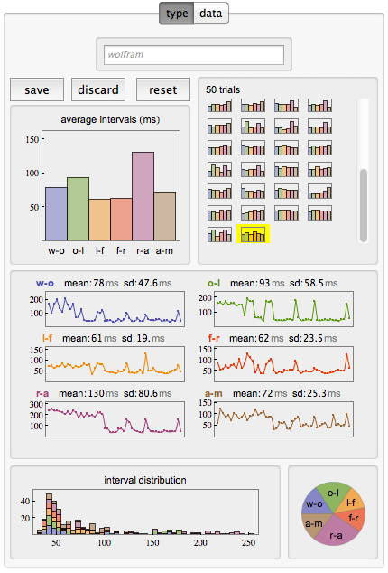
A few weeks ago Paul-Jean Letourneau posted an article on Wolfram’s Blog about using Mathematica to collect and analyze keystroke metrics as a way to identify individuals. The article analyzes how you type, measuring the time intervals between your typing the individual characters using a little interactive widget, collecting and visualizing the data while you repeatedly type in the word “wolfram”.

Keystroke metrics of 50 trials typing the word “wolfram”


It is somewhat interesting at this point to analyze one’s one typing style. For example there appears to be a bi-modal distribution of the time intervals between keystrokes, with the sequence “r-a” taking me almost twice as long (~130ms) as most other sequences (~60-70ms). There is also a ‘learning’ effect visible in my 50 trials, where the speed improves noticeably after about 20 repetitions or so. However, there are occasional relapses into a much slower typing pattern throughout the rest of the trials.

However, what I thought was more interesting is the subsequent analysis the author did across a set of 42 such series he obtained from his colleagues (noting humorously that “it just so happens that Wolfram is a company full of data nerds”). He then proceeds to analyze and visualize that data in various ways.

Distribution Histogram of keystroke intervals

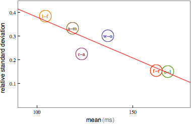
He observes the bimodal nature of the distribution with peaks around 75ms and 150ms for different pairs of characters. In fact, averaging over all those pair typing times, a correlation is found indicating that when people type slower they are more consistent.

(Negative) Correlation of pairwise typing speed and consistency

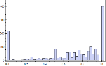
The analysis continues with the observation that each measurement can be seen as a point in a six-dimensional space (six pair-transitions in a word with seven characters). When a person types this same word 50 times you get a cluster of 50 points in six-dimensional space. Different individuals will produce different clusters. So one can use the (built-in) function FindClusters to determine such clusters. However, since people have a certain amount of inconsistency in their typing, it is possible that sometimes one person’s typing will show up in another person’s cluster and vice versa. To measure the quality of the clusters to distinguish individuals, one can implement various measures. The author implements the Rand-index, a measure of the similarity between two data-clusterings. This gives a numeric accuracy on a scale from 0 to 1 for the ability to distinguish between a pair of two people. When looking across all pairs of 42 people – there are 21*41=861 different pairs, but the author chose to look at all 42*42=1764 pairs, as the FindCluster results depend on the sequence input data, so Rand[i,j] may be different from Rand[j,i] – you get the following histogram of Rand quality scores:

Histogram of Rand quality score for all pairs

This clearly shows that keystroke metrics for one word are not sufficient to reliably distinguish between arbitrary pairs of people. The average quality score is only 0.67. On the other hand, about 400 (~23%) of those quality scores are a perfect 1.0, so for about a quarter of the pairs it alone would suffice to reliably distinguish the two people typing. About half as many scores are 0.0, meaning that the clusters overlap so much that no distinction is possible. The remaining scores are distributed mostly between 0.5 and 1.0, meaning you would just guess right more often than wrong.

The author wraps up the post with this paragraph:

Using this fun little typing interface, I feel like I actually learned something about the way my colleagues and I type. The time to type two letters with the same finger on the same hand takes twice as long as with different fingers. The faster you type, the more your typing speed will fluctuate. The more your typing speed fluctuates, the harder it will be to distinguish you from another person based on your typing style. Of course we’ve really just scratched the surface of what’s possible and what would actually be necessary in order to build a keystroke-based authentication system. But we’ve uncovered some trends in typing behavior that would help in building such a system.

An interactive CDF widget embedded in the article allows you to collect and visualize the timing of your own typing. Source code as well as the test data is also shared if you want to further explore the details of this interesting analysis.

 
1 Comment

Posted by on July 20, 2012 in Linguistic, Scientific


Tags: , , , , , ,

London Tube Map and Graph Visualizations

London Tube Map and Graph Visualizations

The previous post on Tube Maps has quickly risen in the view stats into the Top 3 posts. Perhaps it’s due to many people searching Google for images of the original London tube map in the context of the upcoming Olympic Games.

I recently reviewed some of the classes in the free Wolfram’s Data Science course. If you are interested in Data Science, this is excellent material. And if you are using Mathematica, you can download the underlying code and play with the materials.

It just so happens that in the notebook for the Graphs and Networks: Concepts and Applications class there is a graph object for the London subway.

Mathematica Graph object for the London subway

As previously demonstrated in our post on world country neighborhood relationships, Mathematica’s graph objects are fully integrated into the language and there are powerful visualization and analysis functions.

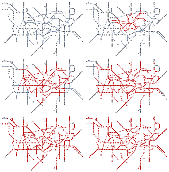
For example, this graph has 353 vertices (stations) and 409 edges (subway connections). This one line of code  highlights all stations no more than 5 stations away from the Waterloo station:

HighlightGraph[london, 
  NeighborhoodGraph[london, "Waterloo", 5]]

Neighborhood Graph 5 around Waterloo

Since HighlightGraph and NeighborhoodGraph are built-in functions, this can be done in one line of code.

Export["london.gif",
  Table[HighlightGraph[london, 
    NeighborhoodGraph[london, "King's Cross St. Pancras", k]],
   {k, 0, 20, 1}]]

creates this animated GIF file:

Paths spreading out from the center

Shortest paths can easily be determined and visualized:

HighlightGraph[london, 
  FindShortestPath[london, "Amersham", "Woolwich Arsenal"]]

A shortest path example

There are many other graph functions such as:

GraphDiameter[london]   39
GraphRadius[london]     20
GraphCenter[london]     "King's Cross St. Pancras"
GraphPeriphery[london]  {"Watford Junction", "Woodford"}

In other words, the King’s Cross St. Pancras station is at the center, with radius up to 20 out into the periphery, and 39 the shortest path between Watford Junction and Woodford, the longest shortest path in the network.

Let’s look at distances within the graph. The built-in function GraphDistanceMatrix calculates all pairwise distances between any two stations:

mat = GraphDistanceMatrix[london]; MatrixPlot[mat]

Graph Distance Matrix Plot

For the 353*353 = 124,609 pairs of stations, let’s plot a histogram of the pairwise distances:

Histogram[Flatten[mat]]

Graph Distance Histogram

The average distance between two stations in the London subway system is about 14.

So far, very little coding has been required as we have used built-in functions. Of course, the set of functions can be easily extended. One interesting aspect is the notion of centrality or distance of a node from the center of the graph. This is expressed in the built-in function ClosenessCentrality

cc = ClosenessCentrality[london];
HighlightCentrality[g_, cc_] := 
   HighlightGraph[g, 
    Table[Style[VertexList[g][[i]], 
      ColorData["TemperatureMap"][cc[[i]]/Max[cc]]], 
        {i, VertexCount[g]}]];
HighlightCentrality[london, cc]

Color coded Centrality Map

Another interesting notion is that of BetweennessCentrality, which is a measure indicating how often a particular node lies on the shortest paths between all node-pairs. The following nifty little snippet of code identifies the 10 most traversed stations – along the shortest paths – of the London underground:

HighlightGraph[london,
 First /@ SortBy[
 Thread[VertexList[london] -> BetweennessCentrality[london]],
 Last][[-10 ;;]]]

10 most traversed stations

I have often felt that progress in computer science and in languages comes from raising the level of abstraction. It’s amazing how much analysis and visualization one can do in Mathematica with very little coding due to the large number of powerful, built-in functions. The reference documentation of these functions often has many useful examples (and is also available for free on the web).
When I graduated from college 20 years ago we didn’t have such powerful language platforms. Implementing a good algorithm for finding shortest paths is a good exercise for a college-level computer science course. And even when such pre-built functions exist, it may still be instructive to figure out how to implement such algorithms.
As manager I have always encouraged my software engineers to spend a certain fraction of their time searching for built-in functions or otherwise pre-existing code to speed up project implementation. Bill Gates has been quoted to have said:

“There is only one trick in software: Use a piece of code that has already been written.”

With software engineers, it is well known that productivity often varies not just by small factors, but by orders of magnitude. A handful of talented and motivated engineers with the right tools can outperform staffs of hundreds at large companies. I believe the increasing levels of abstraction and computational power of platforms such as Mathematica further exacerbates this trend and the resulting inequality in productivity.

 
1 Comment

Posted by on July 11, 2012 in Education, Recreational


Tags: , , , , , , ,

Sankey Diagrams

Sankey Diagrams

Whenever you want to show the flow of a quantity (such as energy or money) through a network of nodes you can use Sankey diagrams:

“A Sankey diagram is a directional flow chart where the width of the streams is proportional to the quantity of flow, and where the flows can be combined, split and traced through a series of events or stages.”
(source: CHEMICAL ENGINEERING Blog)

One area where this can be applied very well is that of costing. By modeling the flow of cost through a company one can analyze the aggregated cost and thus determine the profitability of individual products, customers or channels. Using the principles of activity-based costing one can create a cost-assignment network linking cost pools or accounts (as tracked in the General Ledger) via the employees and their activities to the products and customers. Such a Cost Flow can then be visualized using a Sankey diagram:

Cost Flow from Accounts via Expenses and Activities to Products

The direction of flow (here from left to right) is indicated by the color assignment from nodes to its outflowing streams. Note also the intuitive notion of zero-loss assignment: For each node the sum of the in- and outflowing streams (= height of that node) remains the same. Hence all the cost is accounted for, nothing is lost. If you stacked all nodes on top of one another they would rise to the same height. (Random data for illustration purposes only.)

The above diagram was created in Mathematica using modified source code originally from Sam Calisch who had posted it in 2011 here. Sam also included a “SankeyNotes.pdf” document explaining the details of the algorithms encoded in the source, such as how to arrange the node lists and how to draw the streams.

I find these a perfect example of how a manual drawing can go a long ways to illustrate the ideas behind an algorithm, which makes it a lot easier to understand and reuse the source code. Thanks to Sam for this code and documentation. Sam by the way used the code to illustrate the efficiency of energy use (vs. waste) in Australia:

Energy Flow comparison between New South Wales and Australia (Sam Calisch)

Note the sub-flows within each stream to compare a part (New South Wales) against the whole (Australia).

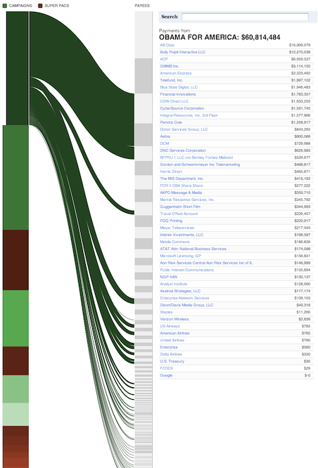
Another interesting use of Sankey Diagrams has been published a few weeks ago on ProPublica about campaign finance flow. This is particularly useful as it is interactive (click on image to get to interactive version).

Tangled Web of Campaign Finance Flow

Note the campaigns in green and the Super-PACs in brown color. The data is sourced from FEC and the New York Times Campaign Finance API. Note that in the interactive version you can click on any source on the left or any destination on the right to see the outgoing and incoming streams.

Finance Flow From Obama-For-America

Finance Flow to American Express

Here are some more examples. Sankey diagrams are also used in Google Flow Analytics (called Event Flow, Goal Flow, Visitor Flow). I wouldn’t be surprised to see Sankey Diagrams make their way into modern data visualization tools such as Tableau or QlikView, perhaps even into Excel some day… Here are some Visio shapes and links to other resources.

 
3 Comments

Posted by on May 14, 2012 in Financial, Industrial


Tags: , , ,

Implementation of TreeMap

Implementation of TreeMap

After posting on TreeMaps twice before (TreeMap of the Market and original post here) I wanted to better understand how they can be implemented.

In his book “Visualize This” – which we reviewed here – author Nathan Yau has a short chapter on TreeMaps, which he also published on his FlowingData Blog here. He is working with the statistical programming language R and uses a library which implements TreeMaps. While this allows for very easy creation of a TreeMap with just a few lines of code, from the perspective of how the TreeMap is constructed this is still a black box.

I searched for existing implementations of TreeMaps in Mathematica (which I am using for many visualization projects). Surprisingly I didn’t find any implementations, despite the 20 year history of both the Mathematica platform and the TreeMap concept. So I decided to learn by implementing a TreeMap algorithm myself.

Let’s recap: A TreeMap turns a tree of numeric values into a planar, space-filling map. A rectangular area is subdivided into smaller rectangles with sizes in relation to the values of the tree nodes. The color can be mapped based on either that same value or some other corresponding value.

One algorithm for TreeMaps is called slice-and-dice. It starts at the top-level and works recursively down to the leaf level of the tree. Suppose you have N values at any given level of the tree and a corresponding rectangle.
a) Sort the values in descending order.
b) Select the first k values (0<k<N) which sum to at least the split-ratio of the values total.
c) Split the rectangle into two parts according to split-ratio along its longer side (to avoid very narrow shapes).
d) Allocate the first k values to the split-off part, the remaining N-k values to the rest of the rectangle.
e) Repeat as long as you have sublists with more than one value (N>1) at current level.
f) For each node at current level, map its sub-tree onto the corresponding rectangle (until you reach leaf level).

As an example, consider the list of values {6,5,4,3,2,1}. Their sum is 21. If we have a split-ratio parameter of say 0.4, then we split the values into {6,5} and {4,3,2,1} since the ratio (6+5)/21 = 0.53 > 0.4, then continue with {6,5} in the first portion of the rectangle and with {4,3,2,1} in the other portion.

Let's look at the results of such an algorithm. Here I'm using a two-level tree with a branching factor of 6 and random values between 0 (dark) and 100 (bright). The animation is iterating through various split-ratios from 0.1 to 0.9:

Notice how the layout changes as a result of the split-ratio parameter. If it’s near 0 or 1, then we tend to get thinner stripes; when it’s closer to 0.5 we get more square shaped containers (i.e. lower aspect ratios).

The recursive algorithm becomes apparent when we use a tree with two levels. You can still recognize the containers from level 1 which are then sub-divided at level 2:

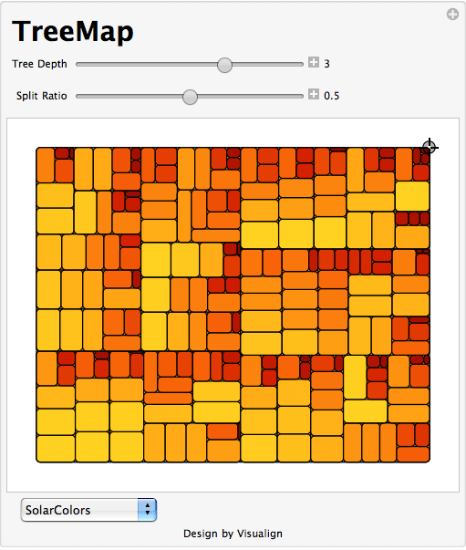
One of the fundamental tenets of this Blog is that interactive visualizations lead to better understanding of structure in the data or of the dynamic properties of a model. You can interact with this algorithm in the TreeMap model in Computable Document Format (CDF). Simply click on the graphic above and you get redirected to a site where you can interact with the model (requires one-time loading of the free CDF Browser Plug-In). You can change the shape of the outer rectangle, adjust the tree level and split-ratio and pick different color-schemes. The values are shown as Tooltips when you hover over the corresponding rectangle. You also have access to the Mathematica source code if you want to modify it further. Here is a TreeMap with three levels:

Of course a more complete implementation would allow to vary the color-controlling parameter, to filter the values and to re-arrange the dimensions as different levels of the tree. Perhaps someone can start with this Mathematica code and take it to the next level. The previous TreeMap post points to several tools and galleries with interactive applications so you can experiment with that.

Lastly, I wanted to point out a good article by the creator of TreeMaps, Ben Shneiderman. In this 2006 paper called “Discovering Business intelligence Using Treemap Visualizations” he cites various BI applications of TreeMaps. Several studies have shown that TreeMaps allow users to recognize certain patterns in the data (like best and worst performing sales reps or regions) faster than with other more traditional chart techniques. No wonder that TreeMaps are finding their way into more and more tools and Dashboard applications.

 
4 Comments

Posted by on November 9, 2011 in Industrial, Scientific


Tags: , , ,

Number of Neighbors for World Countries

Number of Neighbors for World Countries

One important geographical aspect in economy is whether a country is land-locked. Another aspect is the number of neighbors a given country shares a border with. If we sort all 239 world countries, 75 (31%, almost one third) of them are island countries such as Madagascar or Australia where this number is zero. On the opposite end are countries with the most border connections. Here are the top 6 countries in descending order: China (16), Russia (14), Brazil (10), Sudan, Germany, and Democratic Republic of Congo (9 each). All other countries have 8 or less neighbors. Here is a visual breakdown:

The histogram shows the high frequency of island states; the range from 1 to 5 neighbors is fairly common, with a steep drop off in the frequency of 6 or more neighbors. Here is a world map with the same color-code:

WorldMap color-coded by number of neighboring countries

Large countries tend to have more neighbors (Russia (14), China (16), Brazil (10)), but there are obvious exceptions to this tendency (Canada (1), United States (2)). The number of neighbors depends not just on the size of the country itself, but on it’s neighbors’ sizes as well; for example, a small country such as Austria (land area size world rank: 116th) has a rather high number of 8 neighbors because many of them in turn are relatively small (Switzerland, Liechtenstein, Slovenia, etc.).

The average number of neighbors is about 2.7 and there are 323 such border relationships. These can be visualized as graphs with countries as vertices and borders as edges. (Note that to simplify the graphs I excluded all 75 islands = disconnected vertices except Australia.) There are two main partitions of this graph following the land-border geography: One with Europe, Asia and Africa and one with the Americas.

Border-Connected Countries in Europe, Asia, Africa

With the graph layout changed from “Spring Embedding” to “Spring Electrical Embedding” one obtains this interesting variation of the same graph which looks like a sword fish:

The "EurAsiAfrica Sword-fish"

The other partition of the Americas can be visualized in a circular embedding layout:

Europe, Asia, Africa (left) and Americas (right)

It is also interesting to look at the numbers for lengths of pairwise borders between two countries:

  • Number: 323 border-pairs
  • Minimum: 0.34 [km]
  • Maximum: 8893 [km]
  • Mean: 789.6 [km]
  • Total: 255048 [km]
  • Most pairwise borders are between 100 – 1000 km long, but they can as short as 1/3 km (China – Macau) or almost 9000 km (Canada – United States).

    When we look at the entire border length for each country, we see familiar names on top of the ranking:
    China: 22147 [km], Russia: 20293 [km], Brazil: 16857 [km], India: 14103 [km], Kazakhstan: 12185 [km], United States: 12034 [km]. It seems likely that the first four, the so called “BRIC” countries, owe part of their economic strength to their geography: Size, length of borders and number of neighbors influence the number of local trading partners and routes to them. There are many more correlations one can analyze such as between border length / number of neighbors and GDP / length of road network etc. One thing seems likely when it comes to the economy of world countries: Size matters, and so does Geography!

    Epilog: This analysis was all performed using Wolfram’s Mathematica 8. The built-in curated CountryData provides access to more than 200 properties of the world countries, including things like Population, Area, GDP, etc. Some cleaning of the borders lengths data was required to deal with different spellings of the same country. (If you’re interested in the data or source-code, please contact me via email.) List manipulation and mathematical operations such as summation are very easy to do in the functional programming paradigm of Mathematica. Graphs are first-order data structures with numerous vertex and edge operators. Charting is also fairly powerful with BarCharts, ListPlots and more advanced graph charting options. Which other software provides all this flexibility in one integrated package?

     
    6 Comments

    Posted by on October 6, 2011 in Recreational, Socioeconomic


    Tags: , , , ,

    Visualizing Inequality

    Visualizing Inequality

    Measuring and visualizing inequality is often the starting point for further analysis of underlying causes. Only with such understanding can one systematically influence the degree of inequality or take advantage of it. In previous posts on this Blog we have already looked at some approaches, such as the Lorenz-Curve and Gini-Index or the Whale-Curve for Customer Profitability Analysis. Here I want to provide another visual method and look at various examples.

    Inequality is very common in economics. Competitors have different share of and capitalization in a market. Customers have different profitability for a company. Employees have different incomes across the industry. Countries have different GDP in the world economy. Households have different income and wealth in a population.

    The Gini Index is an aggregate measure for the degree of inequality of any given distribution. It ranges from 0.0 or perfect equality, i.e. every element contributes the same amount to 1.0 or the most extreme inequality, i.e. one element contributes everything and all other elements contribute nothing. (The previous post referenced above contains links to articles for the definition and calculation of the Gini index.)

    There are several ways to visualize inequality, including the Lorenz-Curve. Here we look at one form of pie-charts for some discrete distributions. As a first example, consider the distribution of market capitalization among the Top-20 technology companies (Source: Nasdaq, Date: 9/17/11):

    Market Cap of Top 20 Technology Companies on the Nasdaq

    Apple, the largest company by far, is bigger than the bottom 10 combined. The first four (20%) companies – Apple, Microsoft, IBM, Google – are almost half of the entire size and thus almost the size of the other 16 (80%) combined. The pie-chart gives an intuitive sense of the inequality. The Gini Index gives a precise mathematical measure; for this discrete distribution it is 0.47

    Another example is a look at the top PC shipments in the U.S. (Source: IDC, Date: Q2’11)

    U.S. PC Shipments in Q2'11

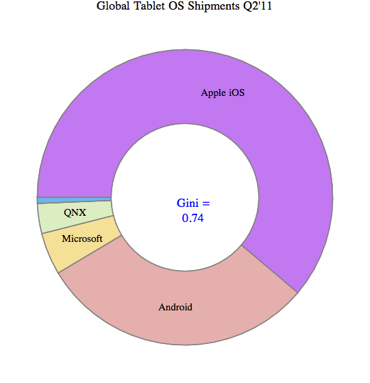
    There is a similar degree of inequality (Gini = 0.46). In fact, this degree of inequality (Gini index ~ 0.5) is not unusual for such distributions in mature industries with many established players. However, consider the tablet market, which is dominated by Apple’s iOS (Source: Strategy Analytics, Date: Q2’11)

    Worldwide Tablet OS shipments in Q2'11

    Apple’s iOS captures 61%, Android 30%, and the other 3 categories combined are under 10%. This is a much stronger degree of inequality with Gini = 0.74

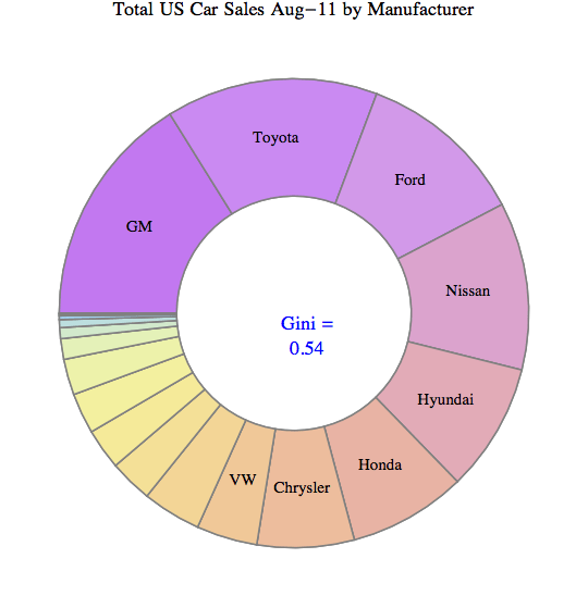
    To pick an example from a different industry, here are the top 18 car brands sold in the U.S. (Source: Market Data Center at WSJ.COM; Date: Aug-2011):

    U.S. Total Car Sales in Aug-11

    When comparing different the Gini index values for these kinds of distributions it is important to realize the impact of the number of elements. More elements in the distribution (say Top-50 instead of Top-20) usually increases the Gini index. This is due to the impact of additional very small players. Suppose for example, instead of the Top-18 you left out the two companies with the smallest sales, namely Saab and Subaru, and plotted only the Top-16. Their combined sales are less than 0.4% of the total, so one wouldn’t expect to miss much. Yet you get a Gini index of 0.49 instead of 0.54. So with discrete distributions and a relatively small number elements one risks comparing apples to oranges when there are different number of elements.

    Consider as a last example a comparison of the above with two other distributions from my own personal experience – the list of base salaries of 30 employees reporting to me at one of my previous companies as well as the list of contributions to a recent personal charity fundraising campaign.

    Gini Index Comparison

    What’s interesting is that the salary distribution has by far the lowest amount of inequality. You wouldn’t believe that from the feelings of employees where many believe they are not getting their fair share and others are getting so much more… In fact, the skills and value contributions to the employer are probably far more unequal than the salaries! (Check out Paul Graham’s essays on “Great Hackers” for more on this topic!)
    And when it comes to donations, the amount people are willing to give to charitable causes differs immensely. We have seen this already in a previous post on Gini-Index with recent U.S. political donations showing an astounding inequality of Gini index = 0.89. I challenge you to find a distribution across so many elements (thousands) which has greater inequality. If you find one, please comment on this Blog or email me as I’d like to know about it.

     
    8 Comments

    Posted by on September 22, 2011 in Industrial, Scientific, Socioeconomic


    Tags: , ,

    Business Benefits of Software Release in Multiple Increments

    One of the main principles of Lean-Agile Software Development is to deliver fast and in small increments. Breaking a large system into multiple increments and delivering some of them early has many benefits to both the business and the customer such as: Earn returns for delivered value sooner. Obtain customer feedback sooner to clarify future features. Capture more market share due to early mover advantage. Reduce risk of obsolescence due to late delivery.

    While these benefits are somewhat intuitive, how can we better illustrate and quantify such benefits? From a financial, cash-flow perspective, there are three main business benefits of switching from one single release to multiple release increments:

    • Sooner Break-Even
    • Smaller Investment
    • Higher Net Return

    A visual model helps to reinforce and quantify them. In the following 4min demonstration I am using a simplified model to illustrate the above benefits:

    The above demonstration is based on the book “Lean-Agile Software Development – Achieving Enterprise Agility” by Alan Shalloway, Guy Beaver and James Trott. (See chapter 2: The Business Case for Agility) I believe that having such dynamic visualizations can help explain these benefits and thus make a more compelling business case for using Lean-Agile Software Development.

    Business Benefits of Two-Increment Release

    Click on the above graphic to interact with the dynamic model using the Wolfram CDF Player.

     
    1 Comment

    Posted by on August 20, 2011 in Industrial


    Tags: , , ,

    Customer Profitability

    Inequality is often at the root of structure and contrasts. Exposing inequality can often lead to insight. For example, take the well-known Pareto principle, which states that roughly 80% of the effects come from 20% of the causes (hence also referred to as the 80-20 rule).

    From the above Wikipedia page on the Pareto principle, chapter on business:

    The distribution shows up in several different aspects relevant to entrepreneurs and business managers. For example:
    80% of your profits come from 20% of your customers
    80% of your complaints come from 20% of your customers
    80% of your profits come from 20% of the time you spend
    80% of your sales come from 20% of your products
    80% of your sales are made by 20% of your sales staff
    Therefore, many businesses have an easy access to dramatic improvements in profitability by focusing on the most effective areas and eliminating, ignoring, automating, delegating or re-training the rest, as appropriate.

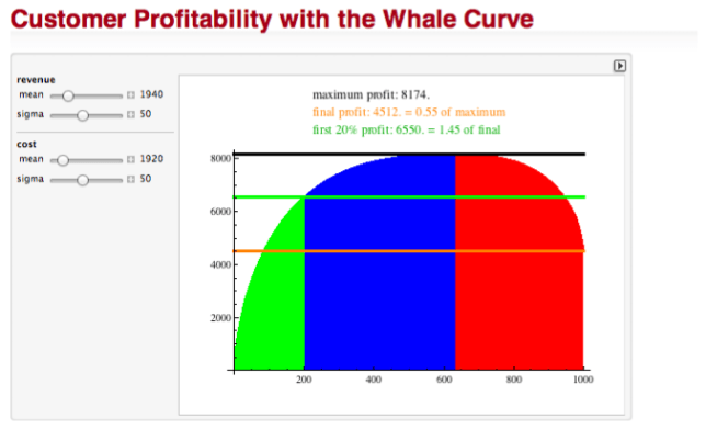
    Visualization can be a powerful instrument for such analysis. For customer profitability, a graphical representation of this inequality is often used as a starting point for analysis. A commonly used visualization is the so-called Whale-Curve. I created a short, 4 min video recording of a dynamic Whale-Curve Demonstration:

    In case you’re curious, the above demonstration uses an underlying model I created in Mathematica. You can dynamically interact with it yourself using the free CDF (Computable Document Format) Player:

    I have provided it as a contribution to the Wolfram Demonstration project, so you can download it, and even look at the source code if you are a Mathematica user.

    If you are interested in applying customer profitability analysis to your business, you may want to consider the company RapidBusinessModeling, which has an elaborate analysis approach starting with such Whale-Curves.

    The underlying notion of Inequality is a fundamental concept. We will look at it in other contexts in a later post.

     
    2 Comments

    Posted by on August 18, 2011 in Financial, Industrial, Scientific


    Tags: , , , ,

     
    %d bloggers like this: